Assignment 3 - Numerical Computations

Ex 1

# Explain
import numpy as np
a = np.array([0., np.finfo(np.float32).eps/2 ]).astype('float32')
print (a.argmax())
print ( (a+1).argmax() )

1
0

Ex 2

# Explain and propose a better solution to compute the variance of the numpy array x
import numpy.random as rand
x = np.array([10000 + rand.random() for i in range(10)]).astype('float32')
variance = np.mean(np.power(x,2,dtype='float32'),dtype='float32') - np.power(np.mean(x, dtype='float32'),2,dtype='float32')
print (variance)
stddev = np.sqrt(variance)

np.std(x)

-8.0

/usr/local/lib/python3.6/dist-packages/ipykernel_launcher.py:5: RuntimeWarning: invalid value encountered in sqrt

”””

0.2364306

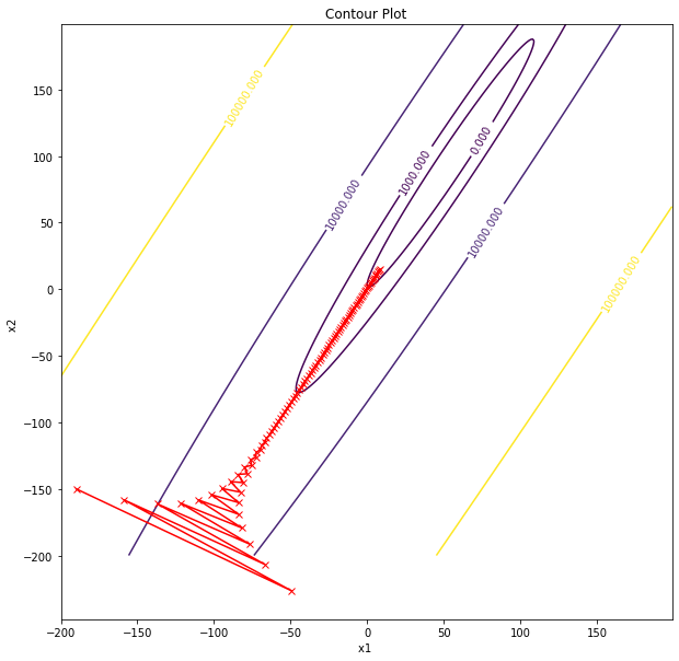
Ex 3

# Take learning rate = 0.18, 0.01, 0.1, 0.2 and explain what's happening when we perform gradient descent
# Why learning rate = 0.1 performs so nicely at the begining of the descent. Justify.

import matplotlib.pyplot as plt


A = np.array ([[0.1,0],[0,10]])
theta = np.pi/3
R = np.array ( [[ np.cos(theta), np.sin(theta)] , [-np.sin(theta), np.cos(theta)]] )
H = np.matmul ( np.matmul (np.transpose(R), A )  , R )  
print (H)

x1_vals = np.arange(-200, 200, 1)
x2_vals = np.arange(-200, 200 , 1)

x1, x2 = np.meshgrid(x1_vals , x2_vals)

z = 7.525/2 * x1**2  + 2.575/2 * x2**2 + -4.32 * x1 * x2 +  -9 * x2 + 15

fig = plt.figure(figsize=(10,10))
ax = plt.axes()
cp = ax.contour(x1, x2, z, [0, 1000, 10000, 100000])
ax.clabel(cp, inline=True, fontsize=10)
ax.set_title('Contour Plot')
ax.set_xlabel('x1 ')
ax.set_ylabel('x2 ')
# ax.set_xlim([-100,-70])
# ax.set_ylim([-200,-150])
# plt.show()

# gradient descent
x1, x2 = -190, -150
eps = 0.18
pts_x1  = [x1]
pts_x2 = [x2]


for i in range (100 ):

  g= np.array ( [(7.525 * x1 -4.32 * x2 ) , (2.575*x2 -4.32 * x1 -9) ])
  gt_h_g = np.dot ( np.dot ( g , H  ) ,  g)
  gt_g = np.dot ( g , g )  
  # print (gt_g/gt_h_g)
  (x1, x2)   =  (x1 - eps * g[0] ,  x2 - eps * g[1] )
  pts_x1.append(x1)
  pts_x2.append(x2)

plt.plot(pts_x1, pts_x2, 'r-x')
plt.show()

[[ 7.525      -4.28682575]
 [-4.28682575  2.575     ]]

Ex 4

# explain what is going wrong, propose a fix
# n.b. you cannot change the hardcoded numbers

def softmax (x):
  return np.exp(x)/np.sum(np.exp(x))

def logloss ( probs, y ):
  return -np.log (np.sum( probs * y))

logits = np.array([89, 50, 60]).astype('float32')
probs = softmax(logits)
y = np.array([1, 0, 0])
loss = logloss ( probs, y )

print (loss)

nan

/usr/local/lib/python3.6/dist-packages/ipykernel_launcher.py:2: RuntimeWarning: overflow encountered in exp

/usr/local/lib/python3.6/dist-packages/ipykernel_launcher.py:2: RuntimeWarning: invalid value encountered in true_divide

Ex 5

# explain what is going wrong, propose a fix

def sigmoid(x):
  return (1/(1+ np.exp(-x)))

def logloss ( prob, y ):
  return -np.log (prob * y)

logit = np.float32(-89)
prob = sigmoid(logit)
y = 1
loss = logloss ( prob, y )

print (loss)

inf

/usr/local/lib/python3.6/dist-packages/ipykernel_launcher.py:4: RuntimeWarning: overflow encountered in exp after removing the cwd from sys.path.

/usr/local/lib/python3.6/dist-packages/ipykernel_launcher.py:7: RuntimeWarning: divide by zero encountered in log import sys

Ex 6

Propose an example of your choice to show why it is worth keeping an eye on numerical computations issues when implementing machine learning algorithms