deeplearninghandbook
Lecture Slides and Programming Exercises that may help study the deep learning book by Goodfellow, Bengio and Courville.
Assignment 4 - Machine Learning Basics
Ex 1
Unsupervised Learning: K-Means
import random as rand
NB_PTS = 100
x1 = [rand.random() for i in range(NB_PTS)]
x2 = [rand.random() for i in range(NB_PTS)]

clustering = [0 for i in range(NB_PTS)]
print (x1)
print (x2)

K = 3
means1 = [rand.random() for i in range(K)]
means2 = [rand.random() for i in range(K)]

def avg(l):
  return sum(l) / len(l)
[0.9471326642214772, 0.3972056462100213, 0.285162711953281, 0.18190518479532058, 0.5064335792294512, 0.09353411577070236, 0.010696628182872203, 0.8931097678552375, 0.25784095683465713, 0.5639077318959898, 0.5827542015346754, 0.9010111760867971, 0.1476923310138849, 0.8723499400325695, 0.616634424038039, 0.7242207521546677, 0.22946996173079803, 0.0930881009256731, 0.5343419877112755, 0.7685347638910641, 0.5195305278653595, 0.4884761910466756, 0.9682856385716665, 0.015981097805567224, 0.7143355260754944, 0.13458893710239128, 0.18773686359287245, 0.713016149743165, 0.9110159736798663, 0.13289237792047692, 0.6365226865007477, 0.021031828837734023, 0.6125128089797299, 0.540631915895912, 0.5066576361894304, 0.5465751532535325, 0.06269782529086254, 0.45665890532842424, 0.36664735889986466, 0.7704328708523737, 0.21740125428848178, 0.5818376040696764, 0.8427066020620296, 0.41704802121417384, 0.8429715197234855, 0.558649778400369, 0.6485213158128974, 0.983759603612089, 0.6343290410107872, 0.6246584863402533, 0.427200174999224, 0.7757066893147263, 0.3256226874918864, 0.05999929880327992, 0.8745417843207866, 0.15395129475382807, 0.8526247017769161, 0.9869040646474659, 0.9720659986235507, 0.30397101369473, 0.08550841865340386, 0.019213777656657327, 0.2984478649947694, 0.006364278604111817, 0.5020050450046293, 0.35244855550138765, 0.9762784154317948, 0.14131968221849656, 0.36153917070333574, 0.7805562706153217, 0.8670940698633243, 0.575626185025867, 0.21958100235207612, 0.6726895692547454, 0.7676458048745965, 0.6388512802643457, 0.826083080901084, 0.6742079058322269, 0.8724131663599253, 0.023329226203601672, 0.010894871758295288, 0.5461391231383529, 0.5230989200208452, 0.7905476385262615, 0.10298448502554602, 0.06832647414099202, 0.712137417191651, 0.33950908414631886, 0.312101677777855, 0.9904438178013495, 0.36491339366954734, 0.8392685976052635, 0.42805252303879004, 0.410365147519657, 0.13365971790981723, 0.9248021445814629, 0.30823262824986997, 0.25147726705488127, 0.680113571140526, 0.4071743956433034]
[0.7259169536261615, 0.8425471305247425, 0.2905783342894377, 0.7732252962477899, 0.7333380847633393, 0.7400985555142192, 0.9506137849196897, 0.8892579457528125, 0.8251580931828051, 0.7587973450936715, 0.5446537069914571, 0.9113590904012822, 0.9436109703764602, 0.007625590585367492, 0.8448412406560851, 0.09064741005648713, 0.7005521230144165, 0.8759977072028418, 0.5720269137674371, 0.5065001022740534, 0.7140260414273187, 0.4432200833130354, 0.33136848918711725, 0.9506674400353428, 0.3073937104296688, 0.27930346052938326, 0.35530231771783627, 0.7391329471248553, 0.5932104626222933, 0.9121822031992429, 0.3230057037570926, 0.8250295138967964, 0.06610551918298546, 0.17314280578032115, 0.3964160924374217, 0.17783724245690458, 0.269874357858389, 0.6860564968465733, 0.24549083807426741, 0.7938316508812853, 0.9864374940900938, 0.4746542152712696, 0.9538950765552364, 0.5300847750525473, 0.8476452673029377, 0.7061465246226748, 0.8564097154133025, 0.6028386791460715, 0.0438212040380781, 0.6727649688098377, 0.6072695340720685, 0.01452724752462542, 0.9362172822211361, 0.09234927491444811, 0.45602954980093535, 0.6245664592208706, 0.3598906135557769, 0.722887509032717, 0.8987712165537107, 0.83923931939261, 0.6256126613007423, 0.19764502032917286, 0.8078809964638973, 0.049791103821660965, 0.15869968480509022, 0.8940000206572345, 0.9771797124112325, 0.4937268490172475, 0.8879002747802412, 0.40981237396937564, 0.5968590833156399, 0.08563001312789098, 0.007560655397781502, 0.8978106277269198, 0.2260201424412397, 0.6352314154583115, 0.3720895398742535, 0.9153795480862008, 0.17395204654780871, 0.1491061921035053, 0.35164936707177774, 0.9572097535843327, 0.6689820806127575, 0.7689420440358603, 0.18891344206250915, 0.9521846349231509, 0.035463768621823766, 0.3936690373797652, 0.7110190322463776, 0.01332660529811891, 0.10658124538927749, 0.6403910771963597, 0.05329739340410844, 0.9524485610931087, 0.811776405169049, 0.5888521941911261, 0.4633060047469658, 0.4351535289307512, 0.643206883278922, 0.44218689017516744]
# To plot the points

from bokeh.models import ColumnDataSource, LabelSet
from bokeh.plotting import figure, output_file
from bokeh.io import output_notebook, push_notebook, show
from bokeh.layouts import row, gridplot
import math


color_list = {0:'red',1:'blue',2:'green'}
family_list = {0:"cluster 0", 1:"cluster 1", 2: "cluster 2"}
marker_list = {0:'x', 1:'o', 2:'square'}

output_notebook()
plots = []

for it in range(1,10):
  p = figure(tools="pan,wheel_zoom,reset,save",

toolbar_location="above",

title="k-Means iteration: "+str(it))
  for label in range(K):
    source1 = ColumnDataSource(data=dict( x1=[ x1[i] for i in range(NB_PTS) if clustering[i]==label ],
                                          x2=[ x2[i]  for i in range(NB_PTS) if clustering[i]==label ] ))

p.scatter(x="x1", y="x2", source=source1, size=8, color=color_list[label], marker=marker_list[label],

legend_label=family_list[label])

    source2 = ColumnDataSource(data=dict( x1= [means1[label]],
                                            x2= [means2[label]]) )

p.scatter(x="x1", y="x2", source=source2, size=14, color=color_list[label], marker=marker_list[label])

  p.legend.location = "top_left"
  plots.append(p)

  # (a) assign points to means
  # WRITE YOUR CODE HERE

  # (b) update means
  # WRITE YOUR CODE HERE

show (gridplot(plots, ncols=3) )

# (c) can you provide an animated visualization to replace the grid of plots ?
# (d) If the points are uniformly drawn, then it is expected that the sizes of the clusters are almost equal,
# provide test code to verify this hypothesis
Ex 2
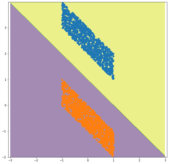
Supervised Learning: SVM
import random as rand
import numpy as np
import matplotlib.pyplot as plt
from sklearn import svm

NB_PTS = 1000
p1 = [rand.random() * 2 -1 for i in range(NB_PTS)]
p2 = [2 - i  + rand.random() for i in p1]

n1 = [rand.random() * 2 -1
for i in range(NB_PTS)]
n2 = [-i - rand.random() for i in n1]

X = list(zip(p1+n1, p2+n2))
Y = [1 for i in range(NB_PTS)] + [-1 for i in range(NB_PTS)]

# (a) what is the analytical solution for the above data using SVM with linear kernel?

clf = svm.SVC(kernel='linear')
clf.fit(X, Y)

# plot the solution
xx, yy = np.meshgrid(np.arange(-3, 3, 0.01),

np.arange(-2, 4, 0.01))

C = np.c_[(xx.ravel(), yy.ravel())]
Z = clf.predict ( C )
Z = Z.reshape(xx.shape)

fig = plt.figure(figsize=(10,10))
ax = plt.axes()


plt.contourf(xx, yy, Z, alpha=0.5)
ax.set_aspect('equal', 'datalim')
ax.scatter(p1, p2)
ax.scatter(n1, n2)
plt.show()

# (b) Extract the solution params form the clf object

# (c) Extract the support vectors from the clf object, can you change the plot to highlight the support vectors?

# (d) Is it possible to use gradient descent to find the optimal SVM solution? Show how, and provide an implementation for this particular example.
# hint: Use the Hinge loss function https://en.wikipedia.org/wiki/Hinge_loss
Ex 3
Cross-Validation
from sklearn.model_selection import train_test_split
from sklearn import datasets
from sklearn import svm
from sklearn.model_selection import cross_val_score

X, y = datasets.load_iris(return_X_y=True)
X_train, X_test, y_train, y_test = train_test_split(X, y, test_size=0.4, random_state=11)

clf = svm.SVC(kernel='rbf')

# There are two parameters for an RBF kernel: C and γ. It is not known beforehand
# which C and γ are best for a given problem; consequently some kind of model selection
# (hyperparameter search) must be done. The goal is to identify good (C, γ) so that the
# classifier can accurately predict unknown data (i.e. testing data).
# We recommend a “grid-search” on C and γ using cross-validation. Various pairs
# of (C, γ) values are tried and the one with the best cross-validation accuracy is
# picked. Reference: https://www.csie.ntu.edu.tw/~cjlin/papers/guide/guide.pdf

# (a) Use cross-validation on (X_train, y_train) to estimate the best hyperparameters C and gamma for the clf classifier
# Do a grid search over C = 2^−5, 2^−3, ..., 2^15 and γ = 2^−15, 2^−13, ... , 2^3).

# (b) What are the default C and γ parameters that are picked automatically by the classifier?
# Do the parameters that you found perform better than the default sklearn parameters?

# (b) what is the final test score

clf
SVC(C=1.0, break_ties=False, cache_size=200, class_weight=None, coef0=0.0,
decision_function_shape=’ovr’, degree=3, gamma=’scale’, kernel=’rbf’, max_iter=-1, probability=False, random_state=None, shrinking=True, tol=0.001, verbose=False)
Ex 4
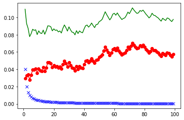
Bias and Variance for K-NN
Consider K-nearest neighbor regression where the true $y$ is coming from a predefined function $f$ and an unavoidable noise $\epsilon$ of mean $0$ and variance $\sigma$
\[y = f(x) + \epsilon\]Consider a fixed given point $x_0$ and a sample $x_1, x_2, …, x_m$. Assume that the values of $x_i$ in the sample are fixed in advance (nonrandom).
We estimate $y_0$ as the value for $x_0$ using the formula:
\[\hat{y}_0 = \frac{1}{k} \sum_{l=1}^k f(x_l)\]where $x_l$ are the closest $k$ neighbors to $x_0$ (in Euclidean distance sense)
The bias for K-NN regression is defined as $f(x_0) - \frac{1}{k} \sum_{l=1}^k f(x_l) $
The variance is $\frac{\sigma^2}{k}$
The error is $\text{Bias}^2 + \text{Var} + \sigma^2$
Plot the three curves of $\text{Bias}^2$, variance and error. Estimate the best parameter $k$ for the following example.
import random as rand
import matplotlib.pyplot as plt
sigma = 0.2
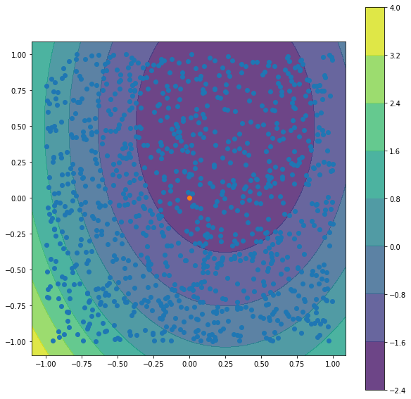
def f(x1, x2):
return 2*x1**2 + x2**2 - x1 -x2 - 2
def avg(l):
return sum(l) / len(l)
NB_PTS = 1000
X1 = [ 2*rand.random()-1 for i in range(NB_PTS) ]
X2 = [ 2*rand.random()-1 for i in range(NB_PTS) ]
x01 = 0
x02 = 0
y0 = f(x01, x02) + rand.normalvariate (0, sigma)
X = list ( zip ( X1, X2) )
# we are trying to estimate the value of f at (0,0) as a mean of f at random surrounding points
fig = plt.figure(figsize=(10,10))
ax = plt.axes()
xx, yy = np.meshgrid(np.arange(-1.1, 1.1, 0.01),
np.arange(-1.1, 1.1, 0.01))
C = np.c_[(xx.ravel(), yy.ravel())]
Z = np.array([f(*i) for i in C ])
Z = Z.reshape(xx.shape)
cf = ax.contourf(xx, yy, Z, alpha=0.8, origin='lower')
ax.set_aspect('equal')
ax.scatter(X1,X2)
ax.scatter([x01],[x02])
fig.colorbar(cf)
plt.show()
from sklearn.neighbors import NearestNeighbors
import numpy as np

# WRITE YOUR CODE HERE