deeplearninghandbook
Lecture Slides and Programming Exercises that may help study the deep learning book by Goodfellow, Bengio and Courville.
Assignment 6: Regularization
Ex 1
Data Augmentation
In this experiment, we aim to classify grocery images. In the same time, it is a first PyTorch tutorial, maybe you will like it even more than TensorFlow or Keras!
We also will experiment with transfer learning since we will use a pre-trained network and only change its output layer!
Show that data augmentation using image transformations improves the generalization performance (testing loss - training loss) of our classifier.
In PyTorch, it is easy to inject random data transformation using the torchvision.transforms module
Try as many transformations as you like and report with your remarks.
Reference: https://pytorch.org/docs/stable/torchvision/transforms.html
# run only one time to download the dataset
! git clone https://github.com/marcusklasson/GroceryStoreDataset.git
Cloning into 'GroceryStoreDataset'...
remote: Enumerating objects: 6553, done.[K
remote: Total 6553 (delta 0), reused 0 (delta 0), pack-reused 6553[K
Receiving objects: 100% (6553/6553), 116.24 MiB | 41.15 MiB/s, done.
Resolving deltas: 100% (313/313), done.
import os
import random
import PIL.Image
import numpy as np
import matplotlib.pyplot as plt

images_path=[]
labels=[]
for dir, subdir, files in os.walk("/content/GroceryStoreDataset/dataset/train/"):
    # print (files)
    for file in files:

images_path.append(os.path.join(dir, file))

labels.append(dir.split('/')[-1])

print (len(labels))
print (len(set(labels)))
2640
81
x, y = random.sample( list ( zip(images_path, labels) ), 1)[0]
im = PIL.Image.open(x)
display(im)
print(y)

Arla-Natural-Yoghurt
import torch
from torchvision import datasets, transforms, models
from torch.utils.data import Dataset, DataLoader

class GroceryDataset(Dataset):
    def __init__(self, root, transform=None):

self.images_path=[]
        self.labels=[]
        for dir, subdir, files in os.walk(root):
          for file in files:

self.images_path.append(os.path.join(dir, file))

self.labels.append(dir.split('/')[-1])
        self.transform = transform
        self.classes = dict ( [ (y,x) for (x,y) in enumerate ( set (self.labels) )  ] ) # no for loops
        # classes ["Arla-Natural-Yoghurt"] = 33


    def __len__(self):
        return len(self.labels)

    def __getitem__(self, idx):

        target = self.classes [ self.labels[idx] ]
        im = PIL.Image.open(self.images_path[idx])
        if self.transform:
          im = self.transform(im)
        else:
          im = transforms.ToTensor()(im)


        return im, target

# data augmentation can be controlled here by adding some random transformations
transform_ = transforms.Compose([

transforms.Resize((224,224)),
    # add some random transformations ??
    # rotate the picture, remove parts of the lectures, add some noise // data augmenation


transforms.ToTensor(),
    # nromalize given means and std deviations

transforms.Normalize((0.4914, 0.4822, 0.4465), (0.2023, 0.1994, 0.2010)),
])

# data augmentation is only used for training, we do not augment the test data
# But to raise the challenge, maybe you can inject a transformation to the test set
transform_test = transforms.Compose([

transforms.Resize((224,224)),
    # nromalize given means and std deviations

transforms.Normalize((0.4914, 0.4822, 0.4465), (0.2023, 0.1994, 0.2010)),
])


data =
GroceryDataset(root="/content/GroceryStoreDataset/dataset/train/", transform=transform_)
loader = torch.utils.data.DataLoader(data, batch_size=64, shuffle=True)

testdata =
GroceryDataset(root="/content/GroceryStoreDataset/dataset/test/", transform=transform_test)
testloader = torch.utils.data.DataLoader(data, batch_size=64, shuffle=True)

# for i in range (3):
#   for x, y in loader:
#     print (x.shape, y)
print (len(data.classes))
print (len(testdata.classes))
81
81
# if it prints cpu, runtime -> change runtime type -> Hardware accelerator -> select gpu
device = torch.device("cuda:0" if torch.cuda.is_available() else "cpu")
print (device)
cuda:0
from torch import nn
from torch import optim


# take the alexnet neural network and change the last layer
model = models.alexnet(pretrained=True)
print (model.classifier[6])
model.classifier[6]= nn.Sequential(

nn.Linear(in_features=4096, out_features=len(data.classes)),

nn.LogSoftmax(dim=1) )

criterion = nn.NLLLoss()

# we just optimize with respect to the last layer weights and biases!
optimizer = optim.Adam(model.classifier[6].parameters(), lr=0.003)

model.to(device)
model
Linear(in_features=4096, out_features=1000, bias=True)
AlexNet(
  (features): Sequential(
    (0): Conv2d(3, 64, kernel_size=(11, 11), stride=(4, 4), padding=(2, 2))
    (1): ReLU(inplace=True)
    (2): MaxPool2d(kernel_size=3, stride=2, padding=0, dilation=1, ceil_mode=False)
    (3): Conv2d(64, 192, kernel_size=(5, 5), stride=(1, 1), padding=(2, 2))
    (4): ReLU(inplace=True)
    (5): MaxPool2d(kernel_size=3, stride=2, padding=0, dilation=1, ceil_mode=False)
    (6): Conv2d(192, 384, kernel_size=(3, 3), stride=(1, 1), padding=(1, 1))
    (7): ReLU(inplace=True)
    (8): Conv2d(384, 256, kernel_size=(3, 3), stride=(1, 1), padding=(1, 1))
    (9): ReLU(inplace=True)
    (10): Conv2d(256, 256, kernel_size=(3, 3), stride=(1, 1), padding=(1, 1))
    (11): ReLU(inplace=True)
    (12): MaxPool2d(kernel_size=3, stride=2, padding=0, dilation=1, ceil_mode=False)
  )
  (avgpool): AdaptiveAvgPool2d(output_size=(6, 6))
  (classifier): Sequential(
    (0): Dropout(p=0.5, inplace=False)
    (1): Linear(in_features=9216, out_features=4096, bias=True)
    (2): ReLU(inplace=True)
    (3): Dropout(p=0.5, inplace=False)
    (4): Linear(in_features=4096, out_features=4096, bias=True)
    (5): ReLU(inplace=True)
    (6): Sequential(
      (0): Linear(in_features=4096, out_features=81, bias=True)
      (1): LogSoftmax()
    )
  )
)
epochs = 10
steps = 0
running_loss = 0


for epoch in range(epochs):
  for inputs, labels in loader:
      # print (inputs.shape)
      steps += 1
      # Move input and label tensors to the default device
      inputs= inputs.to(device)
      labels = labels.to(device)

optimizer.zero_grad()
      logps = model.forward(inputs)
      loss = criterion(logps, labels)
      loss.backward()
      optimizer.step()
      running_loss += loss.item()
  print(f"Epoch {epoch+1}/{epochs}.. "
      f"Train loss: {running_loss/len(loader):.3f}.. ")
  running_loss = 0


test_loss = 0
test_accuracy = 0
model.eval()
with torch.no_grad():
    for inputs_test, labels_test in testloader:
        inputs_test, labels_test = inputs_test.to(device), labels_test.to(device)
        logps_test = model.forward(inputs_test)
        batch_loss = criterion(logps_test, labels_test)
        test_loss += batch_loss.item()
        # Calculate accuracy
        ps = torch.exp(logps_test)
        top_p, top_class = ps.topk(1, dim=1)
        equals = top_class == labels_test.view(*top_class.shape)
        test_accuracy += torch.mean(equals.type(torch.FloatTensor)).item()

print(
      f"Test loss: {test_loss/len(testloader):.3f}.. "
      f"Test accuracy: {test_accuracy/len(testloader):.3f}")

model.train();
Epoch 1/10.. Train loss: 1.778..
Epoch 2/10.. Train loss: 0.415..
Epoch 3/10.. Train loss: 0.307..
Epoch 4/10.. Train loss: 0.240..
Epoch 5/10.. Train loss: 0.188..
Epoch 6/10.. Train loss: 0.157..
Epoch 7/10.. Train loss: 0.208..
Epoch 8/10.. Train loss: 0.189..
Epoch 9/10.. Train loss: 0.141..
Epoch 10/10.. Train loss: 0.151..
Test loss: 0.085.. Test accuracy: 0.972
Ex 2
Adversarial training
In this experiment, we generate adversarial images for the grocery dataset and the model that we just learned using a library called foolbox https://github.com/bethgelab/foolbox
Augmenting the original dataset by these adversarial samples helps the regularization of the training model. Use the following skeleton code to generate adversarial samples, add them to the original dataset and comment on your findings in terms of training and testing accuracy.
# ! pip install foolbox
import random, os
import foolbox as fb
import PIL.Image
import torch
from torchvision import datasets, transforms, models
from torch import nn

device = torch.device("cuda:0")
images_path=[]
labels=[]
for dir, subdir, files in os.walk("/content/GroceryStoreDataset/dataset/train/Packages"):
    # print (files)
    for file in files:

images_path.append(os.path.join(dir, file))

labels.append(dir.split('/')[-1])

classes = dict ( [ (y,x) for (x,y) in enumerate ( set (labels) )  ] )

ims = []
ys = []
first = True
for (x, y) in random.sample( list ( zip(images_path, labels) ), 2):
  y = classes[y]
  im = PIL.Image.open(x)
  im = transforms.Resize((224,224))(im)
  if (first) :
    display(im)
    first = False
  im = transforms.ToTensor()(im)
  ims.append(im)

ys.append(torch.tensor(y))


# print(ys)
# print (torch.stack(ims).shape)
# print (torch.stack(ys).shape)

# to test separately from the model learned in Ex 1:
# model = models.alexnet(pretrained=True)
# print (model.classifier[6])
# model.classifier[6]= nn.Linear(in_features=4096, out_features=len(set(labels)))
# model.to(device)

preprocessing = dict(mean=[0.4914, 0.4822, 0.4465], std=[0.2023, 0.1994, 0.2010], axis=-3)
fmodel = fb.PyTorchModel(model.eval(), bounds=(0, 1), preprocessing=preprocessing)
attack = fb.attacks.FGSM()
# bigger epsilons lead to more corruption in the image
epsilons = [0.01]
_, advs, success = attack(fmodel, torch.stack(ims).to(device), torch.stack(ys).to(device), epsilons=epsilons)

print (success)
for x in advs:
  logps= model.forward(x)
  ps = torch.exp(logps)
  top_p, top_class = ps.topk(1, dim=1)
  print ("adv classes: ", top_class)
  print ("true classes: ", ys)
  im = transforms.ToPILImage()(x[0].to("cpu"))
  display(im)
  im = transforms.ToPILImage()(x[1].to("cpu"))
  # display(im)

tensor([[True, True]], device='cuda:0')
adv classes:  tensor([[75],
        [75]], device='cuda:0')
true classes:  [tensor(28), tensor(3)]

Ex 3
Noise Robustness vs. dropout in the special case of linear regression
(a) Show that adding Gaussian noise with small magnitude to the weights and biases of linear regression (the noise has mean $0$ and variance $\eta « 1$) does not affect the solution of the gradient descent.
(b) Another way of attempting regularization is by adding a dropout layer. Comment on the feasibility and the impact of this approach for the current scenario.
import torch
from torch import nn
device = torch.device("cuda:0" if torch.cuda.is_available() else "cpu")
# A x = b
A = torch.rand(10,3)
A1 = torch.cat ( (A , torch.ones (10,1)), 1 )
sol = torch.rand(4,1)
b = torch.matmul(A1, sol)
# A1,A,b,
sol
tensor([[0.5491],
        [0.4450],
        [0.0859],
        [0.6499]])
# without adding noise
model = nn.Linear(in_features=3, out_features=1)
model.to(device)

criterion = torch.nn.MSELoss()
optimizer = torch.optim.SGD(model.parameters(), lr = 0.05)

epochs = 1000

inputs= A.to(device)
labels = b.to(device)


for epoch in range(epochs):

optimizer.zero_grad()
  preds = model.forward(inputs)
  loss = criterion(preds, labels)

  loss.backward()
  optimizer.step()


model.eval()
preds = model.forward(inputs)
loss = criterion(preds, labels)
print (loss)
model.train()

print (model.bias)
print (model.weight)
tensor(1.3726e-06, device='cuda:0', grad_fn=<MseLossBackward>)
Parameter containing:
tensor([0.6465], device='cuda:0', requires_grad=True)
Parameter containing:
tensor([[0.5496, 0.4467, 0.0899]], device='cuda:0', requires_grad=True)
Ex 4
L2 regularization vs. L1 regularization
(a) Based on the data provided below, design an experiment to show the difference between the solutions to three logistic regression problems:
- the cost function is cross-entropy
- the cost function is cross-entropy + L2 regularization
- the cost function is cross-entropy + L1 regularization
(b) In the three cases (no regularization, L2 regularization and L1 regularization), compare the weights of the first layer with respect to the variances of the corresponding features and the co-variances of these features w.r.t the label
(c) Show that early stopping is equivalent to L2 regularization for some decay coefficient $\alpha$
N.b. some of the code and the data file belong to https://github.com/udacity/deep-learning-v2-pytorch/tree/master/intro-neural-networks/gradient-descent
Preferably use Pytorch, but it is not mandatory
! wget https://raw.githubusercontent.com/udacity/deep-learning-v2-pytorch/master/intro-neural-networks/gradient-descent/data.csv
--2020-04-13 23:16:16--  https://raw.githubusercontent.com/udacity/deep-learning-v2-pytorch/master/intro-neural-networks/gradient-descent/data.csv
Resolving raw.githubusercontent.com (raw.githubusercontent.com)... 151.101.0.133, 151.101.64.133, 151.101.128.133, ...
Connecting to raw.githubusercontent.com (raw.githubusercontent.com)|151.101.0.133|:443... connected.
HTTP request sent, awaiting response... 200 OK
Length: 1778 (1.7K) [text/plain]
Saving to: ‘data.csv’

data.csv            100%[===================>]   1.74K  --.-KB/s    in 0s

2020-04-13 23:16:16 (21.6 MB/s) - ‘data.csv’ saved [1778/1778]
import matplotlib.pyplot as plt
import numpy as np
import pandas as pd
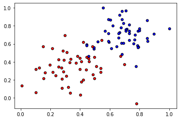
#Some helper functions for plotting and drawing lines
def plot_points(X, y):
admitted = X[np.argwhere(y==1)]
rejected = X[np.argwhere(y==0)]
plt.scatter([s[0][0] for s in rejected], [s[0][1] for s in rejected], s = 25, color = 'blue', edgecolor = 'k')
plt.scatter([s[0][0] for s in admitted], [s[0][1] for s in admitted], s = 25, color = 'red', edgecolor = 'k')
def display(m, b, color='g--'):
plt.xlim(-0.05,1.05)
plt.ylim(-0.05,1.05)
x = np.arange(-10, 10, 0.1)
plt.plot(x, m*x+b, color)
data = pd.read_csv('/content/data.csv', header=None)
X = np.array(data[[0,1]])
y = np.array(data[2])
plot_points(X,y)
plt.show()